The Elixir Telescope
Part 2 : Primary mirror design & calculation

In the last entry I outlined the simulation of an alt-az telescope. I will soon work on the simulator UI. For that, I’ll want a way to simulate focusing. But I have a small problem to tackle first.

A mirror to observe at terrestrial distances

Usually, when it comes to telescopes, your object of interest is located at optical infinity. That means the spherical wavefront coming from it is emitted so far away that from your perspective, the spherical wavefront shell has a radius so big it is a plane. Seen as rays, that means all rays emitted from that point are parallel to each other. They form a parallel beam.

Parabolic mirrors

To focus parallel (on-axis) rays to a single point located at its focal length, a parabolic mirror is a perfect imager. Off-axis, you get an aberration called coma, but ignoring that, you do not have spherical aberration left.

This article understanding foucault, by David A. Harbour explains that quite nicely.

Spherical mirrors

Another option is a spherical mirror, but that only produces a sharp image (without spherical aberration) of an object located at its radius of curvature, and that image is located at its radius of curvature too.

Ellipsoid mirrors

To summarize, up to this point :

• With a conic constant of 0 (spherical), a mirror has two equal distances of interest, equal to its center of curvature.
• When it is accurately parabolic, meaning a conic constant of -1, (we’ll call that 100% corrected, in the sense of corrected of spherical aberration for objects at infinity), it works with a source at infinity and focuses it at its focal length. This focal length is half the paraxial radius of curvature of the mirror.

That means that for my use-case, daylight observing of nearby (20 to 50m) of birds, neither a spherical nor a parabolic mirror will produce an aberration-free on-axis image. Instinct would point to the use of an ellipsoid (conic k where -1 < k < 0).

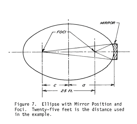
I found an interesting paper on that subject : THE ELLIPSOIDAL MIRROR USED AS AN OBJECTIVE LENS, Robert P. Reedy, Lawrence Livermore Laboratory, Livermore, California

The paper gives an example of an imaging system where an ellipsoidal mirror imaging an object 25 feet away to form an image 27 inches in front of the mirror gave a better image than a parabolic mirror.

Here is a small calculator solving for spherical aberration and best fit conic for nearby objects.

It helps us calculate a few special cases : if we want to observe an object at its radius of curvature (image_distance_from_mirror == curvature_radius, object_distance_from_image == 0), the calculated conic is 0, so a spherical mirror.

If we want to observe a very far object, (object_distance_from_image = 99999999999999999, image_distance_from_mirror == curvature_radius / 2 ), the ideal conic quickly grows to -1, so a parabolic mirror.

For my use-case, let’s say an object distance of 30m, and an image near the focal plane of the equivalent parabolic mirror (so, 400mm), the suggested conic is -0.91, meaning that the optical path difference to correct relative to the nearest sphere is 0.91 times the correction for infinity. To have a more versatile intrument, I’ll just correct it to a parabola.

Let’s add that to the Elixir code to have it around in the future.

defmodule Optics.Ellipsoid do
  @doc """
  Optical Path Difference between a spherical & parabolic surface for light coming from infinity
  """
  def parabolic_opd(radius, curvature_radius),
    do: :math.pow(radius, 4) / (4 * :math.pow(curvature_radius, 3))

  @doc """
  λ/4 criteria
  """
  def rayleigh_limit(wavelength), do: wavelength / 4

  @doc """
  Optical Path Difference between a spherical & ellipsoid surface
  """
  def ellipsoid_opd(radius, curvature_radius, object_distance, image_distance) do
    with opdp <- parabolic_opd(radius, curvature_radius),
         c <- object_distance / 2,
         a <- image_distance + c,
         term2 <- :math.pow(c, 2) / :math.pow(a, 2) do
      opdp * term2
    end
  end

  @doc """
  Best fit conic for a given pair of conjugates, rounded to 2 significant digits
  since that's where I trust my measurements when doing interferometry.
  """
  def best_fit_conic(radius, curvature_radius, obj_dist, img_dist) do
    with opde <- ellipsoid_opd(radius, curvature_radius, obj_dist, img_dist),
         opdp <- parabolic_opd(radius, curvature_radius) do
      Float.round(-1 * opde / opdp, 2)
    end
  end
end

iex(2)> Optics.Ellipsoid.best_fit_conic(57, 800, 50000, 400)
-0.97
iex(3)> Optics.Ellipsoid.best_fit_conic(57, 800, 500000, 400)
-1.0
iex(4)> Optics.Ellipsoid.best_fit_conic(57, 800, 50000, 600)
-0.95
iex(5)> Optics.Ellipsoid.best_fit_conic(57, 800, 10000, 800)
-0.74
iex(7)> Optics.Ellipsoid.best_fit_conic(57, 800, 10000, 400)
-0.86

We can see why I’d rather stay with a parabolic surface at the moment. The conic lowers only for really nearby objects, and quickly goes up again as soon as we want to capture the image near the mirror’s parabolic focal point. If I want the mirror to be usable for faraway objects, it should stay parabolic.

Imaging quality

The camera I’ll use has square pixels of 2.8µm. This is important, because the size of a point source (a star) imaged by a perfect parabolic mirror isn’t a dimensionless point. This wikipedia article about the airy disk summarizes it pretty well. The airy disk radius solely depends on the aperture ratio of the mirror, with the relation r = 1.22λ F/D. Here, λ = 0.000550mm, F = 400mm, D = 114mm, or 2.3µm. The full airy disk then spans 4.6µm for 550nm.

But : as we will work in daylight, there will be a mix of wavelengths, seeing will be quite poor with hot air currents (but we also won’t be traversing a large mass of air), and the huge central obstruction of the mirror will cause a transfer of energy from the airy disk peak to its first and second rings, so we could say that a point source would span a few physical pixels in perfect conditions.

In practice, as we’ve seen earlier, we will have residual spherical aberration from the fact that a parabolic mirror will be used with short object distances, hurting contrast. This is to be expected. For an astronomical telescope, a strehl ratio inferior to 0.9 would be quite disappointing, but it turns out that isn’t too much of a problem for daylight photography.

In other words, a photographic objective is only very rarely diffraction limited.

Those two videos from Huygens Optics do a great job at explaining how hard it is to get maximal MTF from a system that has to work with a wide range of conjugates.

• Huygens Optics, Camera Mirror Lenses pt. 1
• Huygens Optics, Camera Mirror Lenses pt. 2

For the next part, we’ll see what’s yet missing to make a display simulator that takes field of view and depth of field into account, and how an optional barlow lens in the optical path would influence that. We’ll need to raytrace a parabolic mirror.

This virtual display will be replaced by an 1.3” RGB TFT screen on the physical remote control. But we’ll be able to create menus and UIs before I receive it.